Two-Group Comparison

Differential Expression via t-test

Although targeted statistical analyses are beyond the scope of the SomaDataIO package, below is an example analysis that typical users/customers would perform on ‘SomaScan’ data.

It is not intended to be a definitive guide in statistical analysis and existing packages do exist in the R ecosystem that perform parts or extensions of these techniques. Many variations of the workflow below exist, however the framework highlights how one could perform standard preliminary analyses on ‘SomaScan’ data.

Data Preparation

# the `example_data` .adat object
# download from `SomaLogic-Data` repo or directly via bash command:
# `wget https://raw.githubusercontent.com/SomaLogic/SomaLogic-Data/main/example_data.adat`
# then read in to R with:
# example_data <- read_adat("example_data.adat")
dim(example_data)
#> [1]  192 5318

table(example_data$SampleType)
#> 
#>     Buffer Calibrator         QC     Sample 
#>          6         10          6        170

# prepare data set for analysis using `preProcessAdat()`
cleanData <- example_data |>
  preProcessAdat(
    filter.features = TRUE,            # rm non-human protein features
    filter.controls = TRUE,            # rm control samples
    filter.qc       = TRUE,            # rm non-passing qc samples
    log.10          = TRUE,            # log10 transform
    center.scale    = TRUE             # center/scale analytes
  )
#> ✔ 305 non-human protein features were removed.
#> → 214 human proteins did not pass standard QC
#> acceptance criteria and were flagged in `ColCheck`.  These features
#> were not removed, as they still may yield useful information in an
#> analysis, but further evaluation may be needed.
#> ✔ 6 buffer samples were removed.
#> ✔ 10 calibrator samples were removed.
#> ✔ 6 QC samples were removed.
#> ✔ 2 samples flagged in `RowCheck` did not
#> pass standard normalization acceptance criteria (0.4 <= x <= 2.5)
#> and were removed.
#> ✔ RFU features were log-10 transformed.
#> ✔ RFU features were centered and scaled.

# drop any missing values in Sex
cleanData <- cleanData |>
  drop_na(Sex)                         # rm NAs if present

table(cleanData$Sex)
#> 
#>  F  M 
#> 85 83

Compare Two Groups (`M`/`F`)

Get annotations via `getAnalyteInfo()`:

t_tests <- getAnalyteInfo(cleanData) |>
  select(AptName, SeqId, Target = TargetFullName, EntrezGeneSymbol, UniProt)

# Feature data info:
#   Subset via dplyr::filter(t_tests, ...) here to
#   restrict analysis to only certain analytes

t_tests
#> # A tibble: 4,979 × 5
#>    AptName       SeqId     Target              EntrezGeneSymbol UniProt
#>    <chr>         <chr>     <chr>               <chr>            <chr>  
#>  1 seq.10000.28  10000-28  Beta-crystallin B2  CRYBB2           P43320 
#>  2 seq.10001.7   10001-7   RAF proto-oncogene… RAF1             P04049 
#>  3 seq.10003.15  10003-15  Zinc finger protei… ZNF41            P51814 
#>  4 seq.10006.25  10006-25  ETS domain-contain… ELK1             P19419 
#>  5 seq.10008.43  10008-43  Guanylyl cyclase-a… GUCA1A           P43080 
#>  6 seq.10011.65  10011-65  Inositol polyphosp… OCRL             Q01968 
#>  7 seq.10012.5   10012-5   SAM pointed domain… SPDEF            O95238 
#>  8 seq.10014.31  10014-31  Zinc finger protei… SNAI2            O43623 
#>  9 seq.10015.119 10015-119 Voltage-gated pota… KCNAB2           Q13303 
#> 10 seq.10022.207 10022-207 DNA polymerase eta  POLH             Q9Y253 
#> # ℹ 4,969 more rows

Calculate `t-tests`

Use a “list columns” approach via nested tibble object using dplyr, purrr, and stats::t.test()

t_tests <- t_tests |>
  mutate(
    formula = map(AptName, ~ as.formula(paste(.x, "~ Sex"))), # create formula
    t_test  = map(formula, ~ stats::t.test(.x, data = cleanData)),  # fit t-tests
    t_stat  = map_dbl(t_test, "statistic"),            # pull out t-statistic
    p.value = map_dbl(t_test, "p.value"),              # pull out p-values
    fdr     = p.adjust(p.value, method = "BH")         # FDR for multiple testing
  ) |>
  arrange(p.value) |>            # re-order by `p-value`
  mutate(rank = row_number())    # add numeric ranks

# View analysis tibble
t_tests
#> # A tibble: 4,979 × 11
#>    AptName      SeqId Target EntrezGeneSymbol UniProt formula   t_test 
#>    <chr>        <chr> <chr>  <chr>            <chr>   <list>    <list> 
#>  1 seq.8468.19  8468… Prost… KLK3             P07288  <formula> <htest>
#>  2 seq.6580.29  6580… Pregn… PZP              P20742  <formula> <htest>
#>  3 seq.7926.13  7926… Kunit… SPINT3           P49223  <formula> <htest>
#>  4 seq.3032.11  3032… Folli… CGA FSHB         P01215… <formula> <htest>
#>  5 seq.16892.23 1689… Ecton… ENPP2            Q13822  <formula> <htest>
#>  6 seq.9282.12  9282… Cyste… CRISP2           P16562  <formula> <htest>
#>  7 seq.5763.67  5763… Beta-… DEFB104A         Q8WTQ1  <formula> <htest>
#>  8 seq.2953.31  2953… Lutei… CGA LHB          P01215… <formula> <htest>
#>  9 seq.7139.14  7139… SLIT … SLITRK4          Q8IW52  <formula> <htest>
#> 10 seq.4914.10  4914… Human… CGA CGB          P01215… <formula> <htest>
#> # ℹ 4,969 more rows
#> # ℹ 4 more variables: t_stat <dbl>, p.value <dbl>, fdr <dbl>,
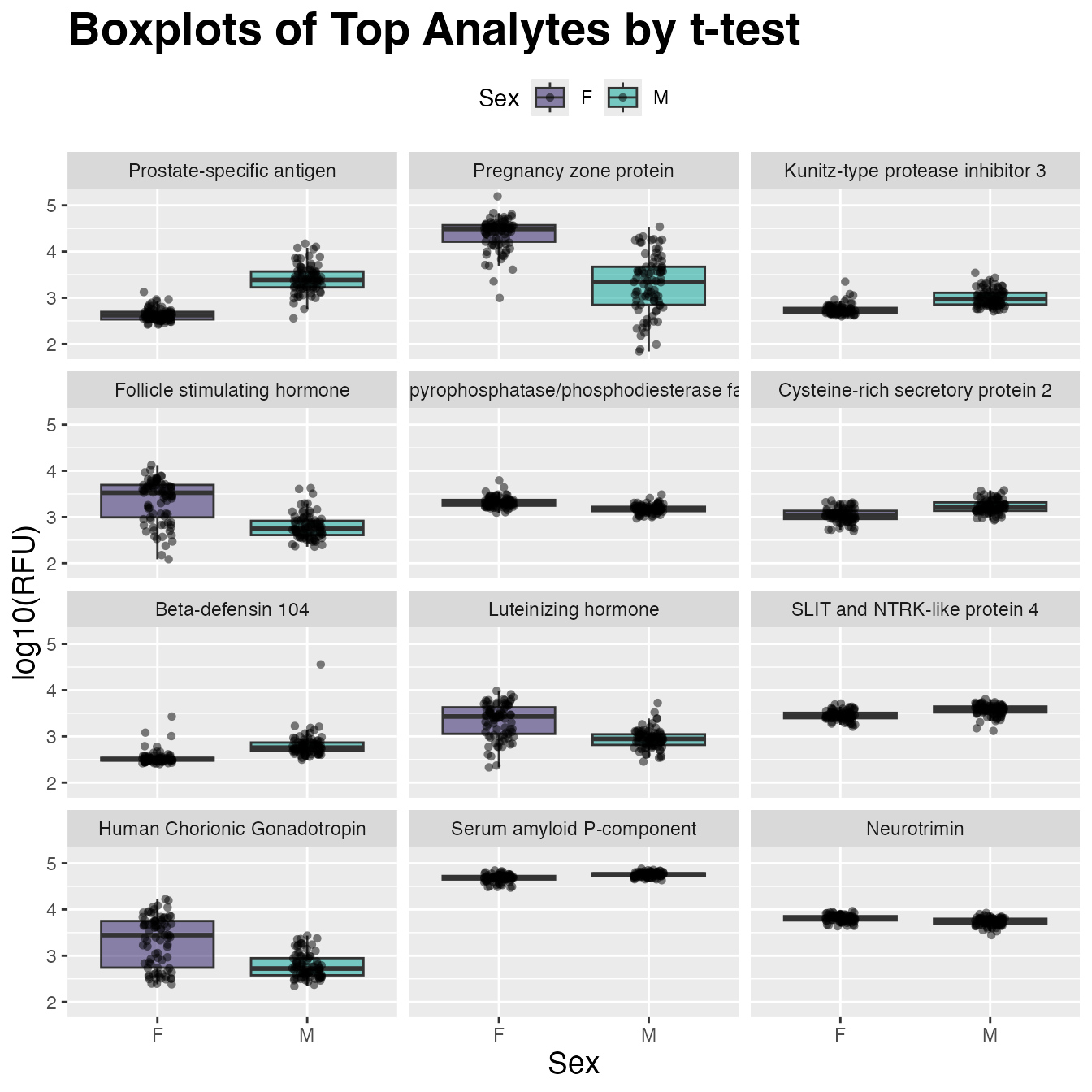
#> #   rank <int>

Visualize with `ggplot2()`

Create a plotting tibble in the “long” format for ggplot2:

target_map <- head(t_tests, 12L) |>     # mapping table
  select(AptName, Target)               # SeqId -> Target

plot_tbl <- example_data |>             # plot non-center/scale data
  filter(SampleType == "Sample") |>     # rm control samples
  drop_na(Sex) |>                       # rm NAs if present
  log10() |>                            # log10-transform for plotting
  select(Sex, target_map$AptName) |>    # top 12 analytes
  pivot_longer(cols = -Sex, names_to = "AptName", values_to = "RFU") |>
  left_join(target_map, by = "AptName") |>
  # order factor levels by 't_tests' rank to order plots below
  mutate(Target = factor(Target, levels = target_map$Target))

plot_tbl
#> # A tibble: 2,040 × 4
#>    Sex   AptName        RFU Target                                     
#>    <chr> <chr>        <dbl> <fct>                                      
#>  1 F     seq.8468.19   2.54 Prostate-specific antigen                  
#>  2 F     seq.6580.29   4.06 Pregnancy zone protein                     
#>  3 F     seq.7926.13   2.66 Kunitz-type protease inhibitor 3           
#>  4 F     seq.3032.11   3.26 Follicle stimulating hormone               
#>  5 F     seq.16892.23  3.44 Ectonucleotide pyrophosphatase/phosphodies…
#>  6 F     seq.9282.12   2.94 Cysteine-rich secretory protein 2          
#>  7 F     seq.5763.67   2.52 Beta-defensin 104                          
#>  8 F     seq.2953.31   2.99 Luteinizing hormone                        
#>  9 F     seq.7139.14   3.43 SLIT and NTRK-like protein 4               
#> 10 F     seq.4914.10   3.93 Human Chorionic Gonadotropin               
#> # ℹ 2,030 more rows

plot_tbl |>
  ggplot(aes(x = Sex, y = RFU, fill = Sex)) +
  geom_boxplot(alpha = 0.5, outlier.shape = NA) +
  scale_fill_manual(values = c("#24135F", "#00A499")) +
  geom_jitter(shape = 16, width = 0.1, alpha = 0.5) +
  facet_wrap(~ Target, ncol = 3) +
  ggtitle("Boxplots of Top Analytes by t-test") +
  labs(y = "log10(RFU)") +
  theme(plot.title = element_text(size = 21, face = "bold"),
        axis.title.x = element_text(size = 14),
        axis.title.y = element_text(size = 14),
        legend.position = "top"
  )

Stu Field, Standard BioTools, Inc.

Differential Expression via t-test

Data Preparation

Compare Two Groups (M/F)

Get annotations via getAnalyteInfo():

Calculate t-tests

Visualize with ggplot2()

Compare Two Groups (`M`/`F`)

Get annotations via `getAnalyteInfo()`:

Calculate `t-tests`

Visualize with `ggplot2()`